The Lennard-Jones Potential

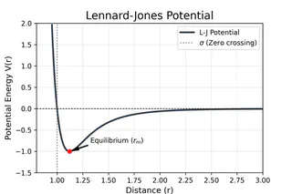
The Lennard-Jones potential (also referred to as the L-J potential or 6-12 potential) is a mathematically simple model that approximates the interaction between a pair of neutral atoms or molecules.

1. The Mathematical Model

The potential energy $V_{LJ}$ is expressed as a function of the distance $r$ between two particles:

Parameters:

• $r$: The distance between the centers of the two particles.
• $\epsilon$ (Epsilon): The depth of the potential well, representing how strongly the particles attract each other.
• $\sigma$ (Sigma): The distance at which the intermolecular potential is exactly zero (often referred to as the “collision diameter”).

2. Physical Meaning of the Terms

The model consists of two distinct parts that compete to determine the stable distance between atoms:

1. The Repulsive Term $\left( \frac{\sigma}{r} \right)^{12}$: This term dominates at short ranges. It represents the Pauli exclusion principle that prevents electrons from occupying the same space, causing atoms to “bounce” off each other.

2. The Attractive Term $\left( \frac{\sigma}{r} \right)^{6}$: This term dominates at long ranges. It represents the Van der Waals forces (specifically London dispersion forces) caused by induced dipole-dipole interactions.

3. Key Characteristics

• Equilibrium Distance: The minimum energy occurs at a distance of $r_m = 2^{1/6}\sigma \approx 1.122\sigma$. At this point, the attractive and repulsive forces are perfectly balanced.
• Applications: It is widely used in molecular dynamics simulations because it is computationally efficient, despite being an approximation.
• Limitation: The $r^{-12}$ power for repulsion is chosen more for computational convenience (it is the square of $r^{-6}$) than for physical precision, as electronic repulsion is more accurately described by an exponential function.

import numpy as np
import matplotlib.pyplot as plt

def lennard_jones(r, epsilon, sigma):
    """Calculate the Lennard-Jones potential."""
    return 4 * epsilon * ((sigma / r)**12 - (sigma / r)**6)

# Parameters for Argon (approximate)
epsilon = 1.0  # Depth of the well
sigma = 1.0    # Distance where potential is zero
r_min = 2**(1/6) * sigma  # Equilibrium distance

# Generate distances (avoiding r=0 to prevent division by zero)
r = np.linspace(0.95 * sigma, 3.0 * sigma, 500)
v = lennard_jones(r, epsilon, sigma)

# Create the plot
plt.figure(figsize=(6, 4))
plt.plot(r, v, color='#2c3e50', linewidth=2.5, label='L-J Potential')

# Add styling and markers
plt.axhline(0, color='black', linestyle='--', linewidth=0.8)
plt.axvline(sigma, color='gray', linestyle=':', label=r'$\sigma$ (Zero crossing)')
plt.scatter([r_min], [-epsilon], color='red', zorder=5)
plt.annotate(f'Equilibrium ($r_m$)', xy=(r_min, -epsilon), xytext=(r_min + 0.2, -epsilon + 0.2),
             arrowprops=dict(facecolor='black', shrink=0.05, width=1, headwidth=5))

# Formatting
plt.title('Lennard-Jones Potential', fontsize=16)
plt.xlabel('Distance (r)', fontsize=12)
plt.ylabel('Potential Energy V(r)', fontsize=12)
plt.ylim(-1.5 * epsilon, 2 * epsilon)
plt.xlim(0.8 * sigma, 3 * sigma)
plt.grid(alpha=0.3)
plt.legend()

# Save the plot for your website (put the PNG in this note's folder: content/notes/2026-02-lennard-jones/)
plt.savefig('lennard_jones_plot.png', dpi=300)
plt.show()

Note: This potential is most accurate for noble gases (like Argon or Neon) but serves as a fundamental building block for modeling more complex molecular systems.